Portfolio risk: drawdown, sizing and daily limits · 4 / 5
Volatility position sizing: stress the lag in an ATR-based rule
A volatility-based sizing rule can increase quantity after a quiet window. If volatility then jumps, that larger position encounters conditions its lagged estimate did not describe. Calculate the rule and the stress loss before treating equal planned risk as equal realized risk.
Athenum7 minUpdated:
Separate a measurement from a forecast
Average True Range measures a smoothed price range using the selected lookback and calculation convention. It is not a directional forecast. An ATR-based stop distance is an explicit strategy choice, not a property that makes a stop safe or an asset likely to reverse.
For the simplified linear contract here, quantity equals cash allowance divided by stop distance. If distance is k × ATR, quantity varies inversely with ATR. In production, include payoff multipliers, costs and quantity increments. Estimate ATR only from data available at the decision time; do not resize a historical trade using the next completed candle.
Add constraints that the volatility rule does not contain
A maximum notional or quantity limit can prevent the rule from expanding without bound when the estimate becomes small. It is an additional policy with its own rationale, not evidence that the volatility forecast is correct. Apply the most restrictive valid quantity across loss, margin, liquidity and notional constraints.
When the observed ATR rises after entry, the original order and stop do not automatically change. Decide in advance whether the strategy holds quantity, reduces it or moves its stop. Widening a stop with unchanged quantity increases the cash risk and must be counted as a new decision.
Worked example: the same budget admits twice the size after calm
Use a hypothetical 100-USDT price-risk allowance, k = 2, and a linear payoff of one USDT per unit per price-unit move. ATR of 5 gives a distance of 10 and quantity 10. ATR of 2.5 gives distance 5 and quantity 20. Both have 100 USDT of planned price risk before costs.
Now assume an adverse execution move of 12 price units before either position exits. The first loses 120 USDT gross, and the second loses 240. A separate cap of 12 units would reduce the calm-window position to 12 units and its shock loss to 144; its original five-unit stop plan would risk only 60. These are hypothetical policy comparisons, not optimal parameters.
| Case | ATR | Quantity | Planned price risk | 12-unit adverse move |
|---|---|---|---|---|
| Normal window | 5 | 10 | 100 | 120 |
| Quiet window | 2.5 | 20 | 100 | 240 |
| Quiet window + size cap | 2.5 | 12 | 60 | 144 |
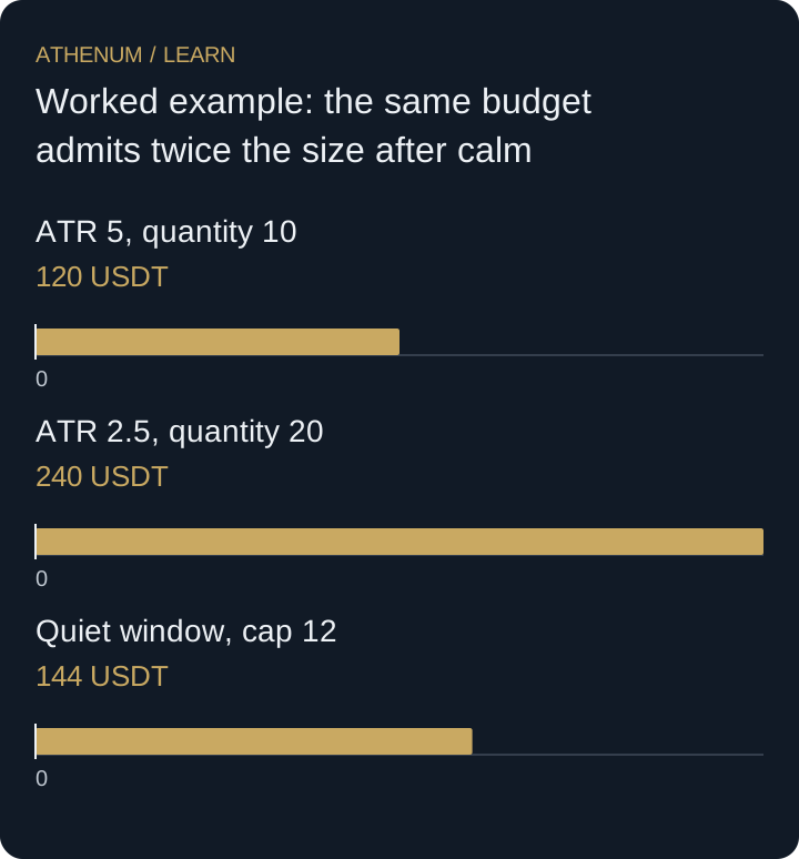 Open full-size diagram
- ATR 5, quantity 10: 120 USDT
- ATR 2.5, quantity 20: 240 USDT
- Quiet window, cap 12: 144 USDT
Do not backfill tomorrow’s risk estimate
If the volatility jump is visible only after the current bar closes, using that higher ATR to reduce the earlier entry size gives the simulation information the trader did not have. Preserve indicator timestamp, order timestamp and actual fill. A smoother risk curve obtained through this timing error is not evidence of a better sizing rule.
Before acting
- Record ATR convention, lookback and last available observation.
- Translate distance into cost-aware executable quantity.
- Apply separate liquidity, notional and margin limits.
- Stress an adverse move before the volatility estimate catches up.
Check your understanding
With a 120-USDT price-risk budget, multiplier 3 and ATR 4, quantity is 10. ATR halves before a later entry. What quantity does the uncapped rule allow, and what is its gross loss for a 15-unit adverse move?
Show the explained answer
The new distance is 3 × 2 = 6, so quantity becomes 120 / 6 = 20. A 15-unit adverse move loses 20 × 15 = 300 USDT gross, 2.5 times the planned price-risk amount. Fees and execution details can increase or change the realized loss.